Example for a latent class analysis with the poLCA-package in R

rstats

latent class analysis

ggplot2

A worked example of polytomous latent class analysis with the poLCA package: fitting the models, comparing model fit, and plotting the classes with ggplot2.

Author

Niels Ohlsen

Published

August 13, 2015

When you work with R for some time, you really start to wonder why so many R packages have some kind of pun in their name. Intended or not, the poLCA package is one of them. Today i´ll give a glimpse on this package, which doesn´t have to do anything with dancing or nice dotted dresses.

This article is kind of a draft and will be revised anytime.

The „poLCA“-package has its name from „Polytomous Latent Class Analysis“. Latent class analysis is an awesome and still underused (at least in social sciences) statistical method to identify unobserved groups of cases in your data. Polytomous latent class analysis is applicable with categorical data. The unobserved (latent) variable could be different attitude-sets of people which lead to certain response patterns in a survey. In marketing or market research latent class analysis could be used to identify unobserved target-groups with different attitude structures on the basis of their buy-decisions. The latent classes are assumed to be nominal. The poLCA package is not capable of sampling weights, yet.

By the way: There is also another package for latent class models called „lcmm“ and another one named „mclust“.

What does a latent class analysis try to do? A latent class model uses the different response patterns in the data to find similar groups. It tries to assign groups that are „conditional independent“. That means, that inside of a group the correlations between the variables become zero, because the group membership explains any relationship between the variables.

Latent class analysis is different from latent profile analysis, as the latter uses continous data and the former can be used with categorical data. Another important aspect of latent class analysis is, that your elements (persons, observations) are not assigned absolutely, but on probability. So you get a probability value for each person to be assigned to group 1, group 2, […], group k.

Before you estimate your LCA model you have to choose how many groups you want to have. You aim for a small number of classes, so that the model is still adequate for the data, but also parsimonious. If you have a theoretically justified number of groups (k) you expect in your data, you perhaps only model this one solution. Another, more exploratory, approach would be to compare multiple models and compare these models against each other. You could compare the different solutions by BIC or AIC information criteria. BIC is preferred over AIC in latent class models, but usually both are used. A smaller BIC is better than a bigger BIC. Next to AIC and BIC you also get a Chi-Square goodness of fit. I once asked Drew Linzer, the developer of poLCA, if there would be some kind of LMR-Test (like in MPLUS) implemented anytime. He said, that he wouldn´t rely on statistical criteria to decide which model is the best, but he would look which model has the most meaningful interpretation and has a better answer to the research question.

Latent class models belong to the family of (finite) mixture models. The parameters are estimated by the EM-Algorithm. It´s called EM, because it has two steps: An „E“stimation step and a „M“aximization step. In the first one, class-membership probabilities are estimated (the first time with some starting values) and in the second step those estimates are altered to maximize the likelihood-function. Both steps are iterative and repeated until the algorithm finds the global maximum. That´s why starting values in latent class analysis are important. If you run the estimation multiple times with different starting values and it always comes to the same solution, you can be pretty sure that you found the global maximum.

data preparation Latent class models don´t assume the variables to be continous, but (unordered) categorical. The variables are not allowed to contain zeros, negative values or decimals as you can read in the poLCA vignette. If your variables are binary 0/1 you should add 1 to every value, so they become 1/2. If you have NA-values, you have to recode them to a new category. Rating Items with values from 1-5 could be added a value 6 from the NAs.

mydata[is.na(mydata)] <- 6

Running LCA models First you should install the package and define a formula for the model to be estimated.

install.packages("poLCA")
library("poLCA")

# By the way, for all examples in this article, you´ll need some more packages:
library("reshape2")
library("plyr")
library("dplyr")
library("poLCA")
library("ggplot2")
library("ggparallel")
library("igraph")
library("tidyr")
library("knitr")

# these are the defaults of the poLCA command
poLCA(formula, data, nclass=2, maxiter=1000, graphs=FALSE, tol=1e-10, na.rm=TRUE, probs.start=NULL, nrep=1, verbose=TRUE, calc.se=TRUE)

#estimate the model with k-classes
k<-3
lc<-poLCA(f, data, nclass=k, nrep=30, na.rm=FALSE, Graph=TRUE)

The following code runs a sequence of models with two to ten groups. With nrep=10 it runs every model 10 times and keeps the model with the lowest BIC.

# select variables
mydata <- data %>% dplyr::select(F29_a,F29_b,F29_c,F27_a,F27_b,F27_e,F09_a, F09_b, F09_c)

# define function
f<-with(mydata, cbind(F29_a,F29_b,F29_c,F27_a,F27_b,F27_e,F09_a, F09_b, F09_c)~1)

#------ run a sequence of models with 1-10 classes and print out the model with the lowest BIC
max_II <- -100000
min_bic <- 100000
for(i in 2:10){
  lc <- poLCA(f, mydata, nclass=i, maxiter=3000,
              tol=1e-5, na.rm=FALSE,
              nrep=10, verbose=TRUE, calc.se=TRUE)
  if(lc$bic < min_bic){
    min_bic <- lc$bic
    LCA_best_model<-lc
  }
}
LCA_best_model

You´ll get the standard-output for the best model from the poLCA-package (conditional item response probabilities by class, estimated class population shares, predicted class memberships, and fit measures AIC/BIC/G^2/X2).

Estimated class population shares
 0.2792 0.4013 0.3195

Predicted class memberships (by modal posterior prob.)
 0.2738 0.4055 0.3206

Fit for 3 latent classes:
number of observations: 577
number of estimated parameters: 155
residual degrees of freedom: 422
maximum log-likelihood: -6646.732
AIC(3): 13603.46
BIC(3): 14278.93
G^2(3): 6121.357
X^2(3): 8967872059

Generate table showing fitvalues of multiple models Now i want to build a table for comparison of various model-fit values (log-likelihood, resid. df, BIC, aBIC, cAIC, likelihood-ratio, Entropy).

#select data
mydata <- data %>% dplyr::select(F29_a,F29_b,F29_c,F27_a,F27_b,F27_e,F09_a, F09_b, F09_c)

# define function
f<-with(mydata, cbind(F29_a,F29_b,F29_c,F27_a,F27_b,F27_e,F09_a, F09_b, F09_c)~1)

## models with different number of groups without covariates:
set.seed(01012)
lc1<-poLCA(f, data=mydata, nclass=1, na.rm = FALSE, nrep=30, maxiter=3000) #Loglinear independence model.
lc2<-poLCA(f, data=mydata, nclass=2, na.rm = FALSE, nrep=30, maxiter=3000)
lc3<-poLCA(f, data=mydata, nclass=3, na.rm = FALSE, nrep=30, maxiter=3000)
lc4<-poLCA(f, data=mydata, nclass=4, na.rm = FALSE, nrep=30, maxiter=3000)
lc5<-poLCA(f, data=mydata, nclass=5, na.rm = FALSE, nrep=30, maxiter=3000)
lc6<-poLCA(f, data=mydata, nclass=6, na.rm = FALSE, nrep=30, maxiter=3000)

# generate dataframe with fit-values
results <- data.frame(Modell=c("Modell 1"),
                      log_likelihood=lc1$llik,
                      df = lc1$resid.df,
                      BIC=lc1$bic,
                      ABIC=  (-2*lc1$llik) + ((log((lc1$N + 2)/24)) * lc1$npar),
                      CAIC = (-2*lc1$llik) + lc1$npar * (1 + log(lc1$N)),
                      likelihood_ratio=lc1$Gsq)
results$Modell<-as.integer(results$Modell)
results[1,1]<-c("Modell 1"); results[2,1]<-c("Modell 2"); results[3,1]<-c("Modell 3")
results[4,1]<-c("Modell 4"); results[5,1]<-c("Modell 5"); results[6,1]<-c("Modell 6")
# ... (llik, resid.df, bic, abic, caic, Gsq filled per model lc2..lc6)

Now i calculate the Entropy (a pseudo-r-squared) for each solution. I took the idea from Daniel Oberski´s Presentation on LCA.

entropy<-function (p) sum(-p*log(p))

results[1,8]<-c("-")
error_prior<-entropy(lc2$P)            # class proportions model 2
error_post<-mean(apply(lc2$posterior,1, entropy),na.rm = TRUE)
results[2,8]<-round(((error_prior-error_post) / error_prior),3)
# ... repeat for lc3..lc6

colnames(results)<-c("Model","log-likelihood","resid. df","BIC","aBIC","cAIC","likelihood-ratio","Entropy")
lca_results<-results

# show as HTML table for copy & paste
install.packages("ztable")
ztable::ztable(lca_results)

Elbow-Plot

install.packages("forcats")
library("forcats")
results$model <- as_factor(results$model)

#convert to long format
results2<-tidyr::gather(results,Kriterium,Guete,4:7)

#plot
fit.plot<-ggplot(results2) +
  geom_point(aes(x=Model,y=Guete),size=3) +
  geom_line(aes(Model, Guete, group = 1)) +
  theme_bw()+
  labs(x = "", y="", title = "") +
  facet_grid(Kriterium ~. ,scales = "free") +
  theme_bw(base_size = 16, base_family = "") +
  theme(panel.grid.major.x = element_blank(),
        panel.grid.major.y = element_line(colour="grey", size=0.5),
        axis.line = element_line(colour = "black"))
fit.plot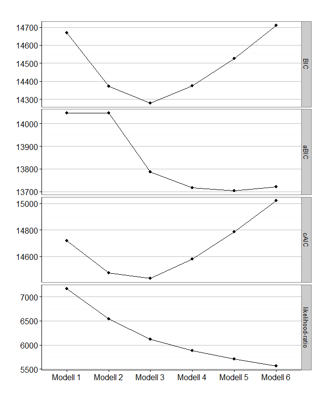

Inspect population shares of classes

round(colMeans(lc$posterior)*100,2)
# [1] 27.92 40.13 31.95

table(lc$predclass)
#   1   2   3
# 158 234 185

round(prop.table(table(lc$predclass)),4)*100
#    1     2     3
# 27.38 40.55 32.06

Ordering of latent classes Latent classes are unordered, so which latent class becomes number one, two, three… is arbitrary. There is a function for manually reordering: poLCA.reorder().

#extract starting values from our previous best model (with 3 classes)
probs.start<-lc3$probs.start

#re-run the model, this time with "graphs=TRUE"
lc<-poLCA(f, mydata, nclass=3, probs.start=probs.start,graphs=TRUE, na.rm=TRUE, maxiter=3000)

# reorder them (Class 1 stays 1, Class 3 becomes 2, Class 2 becomes 1)
new.probs.start<-poLCA.reorder(probs.start, c(1,3,2))

#run polca with adjusted ordering
lc<-poLCA(f, mydata, nclass=3, probs.start=new.probs.start,graphs=TRUE, na.rm=TRUE)

saveRDS(lc$probs.start,"/lca_starting_values.RData")

Plotting This is the poLCA-standard Plot for conditional probabilites (graph=TRUE). It´s in a 3D-style which is not really my taste. I found some code at dsparks on github that makes very appealing ggplot2-plots:

lcmodel <- reshape2::melt(lc$probs, level=2)
zp1 <- ggplot(lcmodel,aes(x = L1, y = value, fill = Var2))
zp1 <- zp1 + geom_bar(stat = "identity", position = "stack")
zp1 <- zp1 + facet_grid(Var1 ~ .)
zp1 <- zp1 + scale_fill_brewer(type="seq", palette="Greys") +theme_bw()
zp1 <- zp1 + labs(x = "Fragebogenitems",y="Anteil der Item-\nAntwortkategorien", fill ="Antwortkategorien")
zp1 <- zp1 + theme(axis.text.y=element_blank(), axis.ticks.y=element_blank(), panel.grid.major.y=element_blank())
zp1 <- zp1 + guides(fill = guide_legend(reverse=TRUE))
print(zp1)

If you want to compare the items directly:

zp2 <- ggplot(lcmodel,aes(x = Var1, y = value, fill = Var2))
zp2 <- zp2 + geom_bar(stat = "identity", position = "stack")
zp2 <- zp2 + facet_wrap(~ L1)
zp2 <- zp2 + scale_x_discrete("Fragebogenitems", expand = c(0, 0))
zp2 <- zp2 + scale_y_continuous("Wahrscheinlichkeiten \nder Item-Antwortkategorien", expand = c(0, 0))
zp2 <- zp2 + scale_fill_brewer(type="seq", palette="Greys") + theme_bw()
zp2 <- zp2 + labs(fill ="Antwortkategorien")
zp2 <- zp2 + theme(axis.text.y=element_blank(), axis.ticks.y=element_blank(), panel.grid.major.y=element_blank())
zp2 <- zp2 + guides(fill = guide_legend(reverse=TRUE))
print(zp2)

Images in original: Antwortprofile_medien_F27_F29_KWB_Variante_A/B/C.png