Multiple Imputation in R. How to impute data with MICE for lavaan.
Missing data is unavoidable in most empirical work. This can be a problem for any statistical analysis that needs data to be complete. Structural equation modeling and confirmatory factor analysis are such methods that rely on a complete dataset. The following post will give an overview on the background of missing data analysis, how the missingness can be investigated, how the R-package MICE for multiple imputation is applied and how imputed data can be given to the lavaan-package for confirmatory factor analysis.
If you are in a hurry and already know the background of multiple imputation, jump to: How to use multiple imputation with lavaan
What kinds of missing data are there? There are two types of missingness: Unit nonresponse concerns cases in the sample, that didn´t respond to the survey at all, or – more generally spoken – the failure to obtain measurements for a sampled unit. Item nonresponse occurs, when a person leaves out particular items in the survey, or – more generally spoken – particular measurements of a sampled unit are missing. Here, we will focus on item nonresponse.
Why is it important? The topic of missing data itself is still often missing in the curriculum of statistics for social sciences and sociology. Also in practical research a lot of studies don´t show transparently how they handled missing data. But there would be a lot reason to pay more attention to this issue. As an example, Ranjit Lall examined how political science studies dealed with missing data and found out, that 50 % had their key results „disappear“ after he re-analysed them with a proper way to handle the missingness: How multiple Imputation makes a difference. Most of these studies used listwise deletion, because it once was a standard way to deal with missings and still is in many software packages. For example, the statistic software SPSS still doesn´t offer multiple imputation (only single imputation with EM-algorithm, that doesn´t incorporate uncertainty and should only be used with a trivial amount of missingness of < 5 %).
DON´T (bad practice) In listwise deletion every observation (every row in the dataset respectively every person in the survey) that has at least one missing value will be dropped completely out of the analysis. Only complete cases are analysed. Another way is pairwise deletion, which often is used for correlations. Here, all cases without missings in the analysed variables are included. The problem is, that if you run a correlation of variable a and variable b, and a correlation of variable a and variable c, your results can be based on a different amount of cases (N). Listwise and pairwise deletion are problematic in multiple ways: both reduce your samplesize and your statistical power decreases. Other studies acknowledge this problem and replace missing values with the mean value of the remaining datapoints (mean value replacement). This is problematic as well, because your standard deviation increases and your results become biased as well.
DO: (state of the art) The state of the Art methods of dealing with missing data (at least in structural equation modeling) are multiple imputation as well as full information maximum likelihood (FIML). In FIML no data is imputed. Instead, an algorithm is used in your analysis (i.e. regression, structural equation modelling) that estimates your model and the missing values in one step, based on your model and all observed data in your sample. FIML should not be confused with EM-Imputation. In multiple imputation each missing value is replaced (imputed) multiple times through a specified algorithm, that uses the observed data of every unit to find a plausible value for the missing cell. Every time a missing value is replaced through an estimated value, some uncertainty/randomness is introduced. This way, each of the resulting datasets differs a little bit, which brings the advantage of a more adequate estimation of variances.
How to use multiple imputation in practice It is the decision of the researcher how many times the cells with missing data are imputed. There are rules of thumb and simulation studies to guide this decision. Often a minimum of 5 imputed datasets is enough, but some researchers think it should depend on the amount of missingness. At some point a greater number of imputation becomes obsolete.
Multiple Imputation needs multivariate normality of the data and the missings ´should at least be MAR (missing at random). Simulation studies showed, that deviation of multivariate normality is not too problematic and even if the data is not MAR, multiple imputation showed itself as robust. Especially in comparison to listwise or pairwise deletion, multiple imputation produces more adequate results in spite of erroneous assumption of MAR or multivariate normality.
There are a lot of tools to do multiple imputation. The standalone Software NORM now also has an R-package NORM for R. Another R-package worth mentioning is Amelia. Now, we turn to the R-package MICE („multivariate imputation by chained equations“) which offers many functions to generate imputed datasets based on your missing data. MICE uses the pmm algorithm which stands for predictive mean modeling that produces good results with non-normal data.
Three types of missingness There are three possible patterns of missingness: – MCAR (Missing completely at random) – MAR (Missing at random) – NMAR (Not missing at random)
To find out if your data is MCAR there is a statistical test called „little´s mcar test“, which tests the null hypothesis that data is completely missing at random. So you want it to be nonsignificant. Problem is, that it’s an omnibus test. The “MissMech” package in R has tests to show if assumptions are met. Little´s MCAR-test is part of the „BaylorEdPsych“ Package.
Let´s do a „Little´s test“ on MCAR:
#--------------------------------------------------
# Little-test
#--------------------------------------------------
install.packages('BaylorEdPsych', dependencies=TRUE)
library(BaylorEdPsych)

# read example data
data(EndersTable1_1)

# run MCAR test
test_mcar<-LittleMCAR(EndersTable1_1)

# print p-value of mcar-test
print(test_mcar$p.value)
As a result we get
print(test_mcar$p.value)
[1] 0.01205778
which means, that the result is significant. The null-hypotheses, that our data is mcar, is rejected. Data is mcar if p > 0.05. There is a possibility, that the test failed, because the data are not normal and homoscedastic. We test this:
install.packages("MissMech")
library("MissMech")

#test of normality and homoscedasticity
out<-TestMCARNormality(EndersTable1_1)
print(out)
Visualisation of missing data patterns
library("dplyr")
#First: Check your missings:
# Proportion of Missingness
propmiss <- function(dataframe) {
  m <- sapply(dataframe, function(x) {
    data.frame(
      nmiss=sum(is.na(x)),
      n=length(x),
      propmiss=sum(is.na(x))/length(x)
    )
  })
  d <- data.frame(t(m))
  d <- sapply(d, unlist)
  d <- as.data.frame(d)
  d$variable <- row.names(d)
  row.names(d) <- NULL
  d <- cbind(d[ncol(d)],d[-ncol(d)])
  return(d[order(d$propmiss), ])
}

miss_vars<-propmiss(EndersTable1_1)
miss_vars_mean<-mean(miss_vars$propmiss)
miss_vars_ges<- miss_vars  %>% arrange(desc(propmiss))

plot1<-ggplot(miss_vars_ges,aes(x=reorder(variable,propmiss),y=propmiss*100)) +
  geom_point(size=3) +
  coord_flip() +
  theme_bw() + xlab("") +ylab("Missingness per variable") +
  theme(panel.grid.major.x=element_blank(),
        panel.grid.minor.x=element_blank(),
        panel.grid.major.y=element_line(colour="grey60",linetype="dashed")) +
  ggtitle("Percentage of missingness")
plot1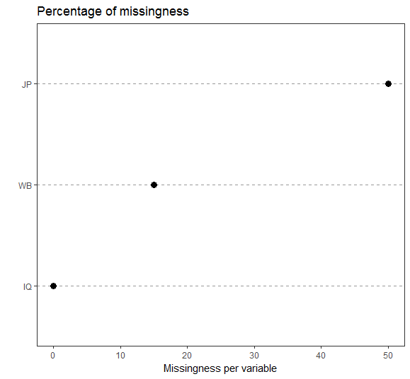
There is no general rule on how much missing data is acceptable. It depends on your research context.
Now, we´ll use the VIM package to visualize missings and if there are any patterns.
install.packages("VIM", dependencies = TRUE)
install.packages("VIMGUI", dependencies = TRUE)
library("VIM")
library("VIMGUI")
VIMGUI()

# If you don´t like to use the GUI because of reproducibility, you can also use the console:
aggr(EndersTable1_1, numbers=TRUE, prop=TRUE, combined=TRUE, sortVars=FALSE, vscale = 1)
After we chose our dataframe from the environment, VIM gives us some plots to visualise our data:
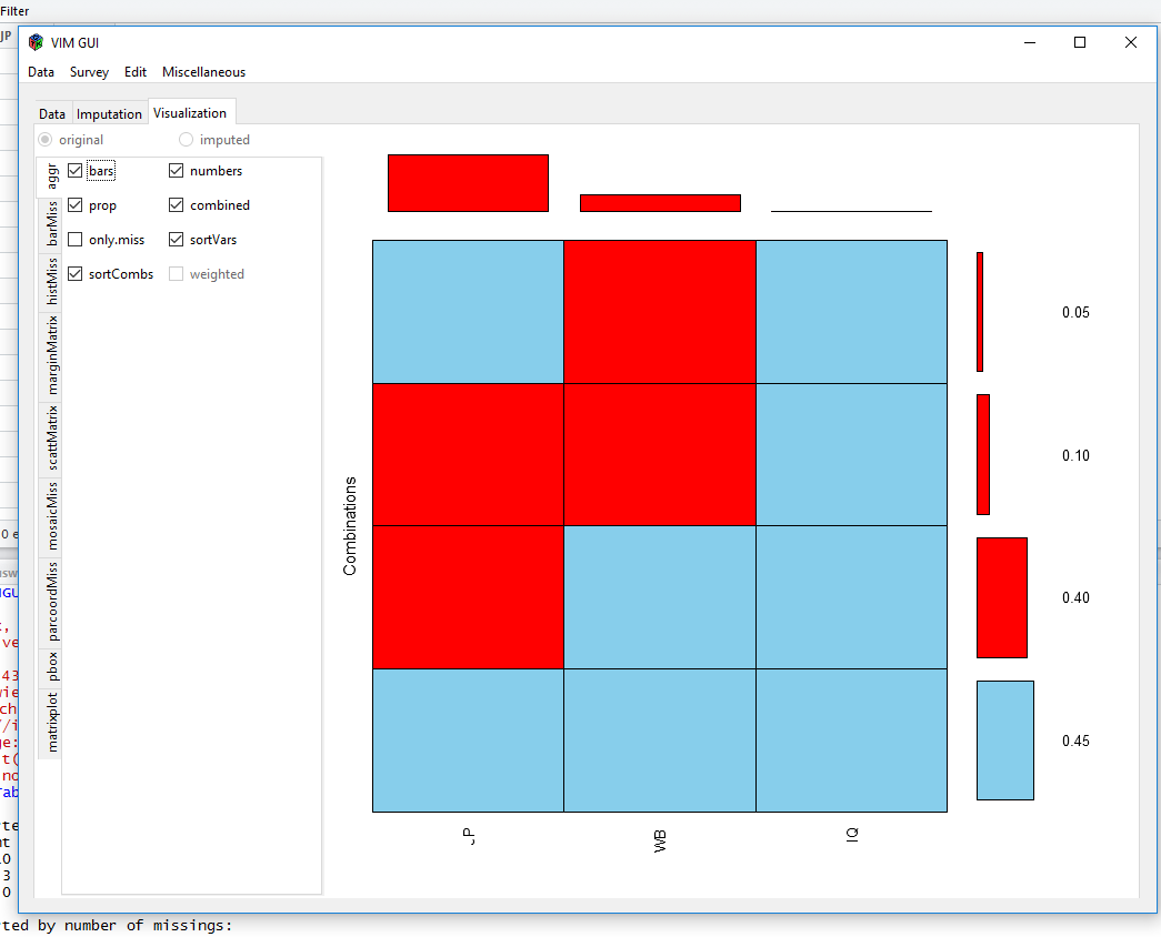
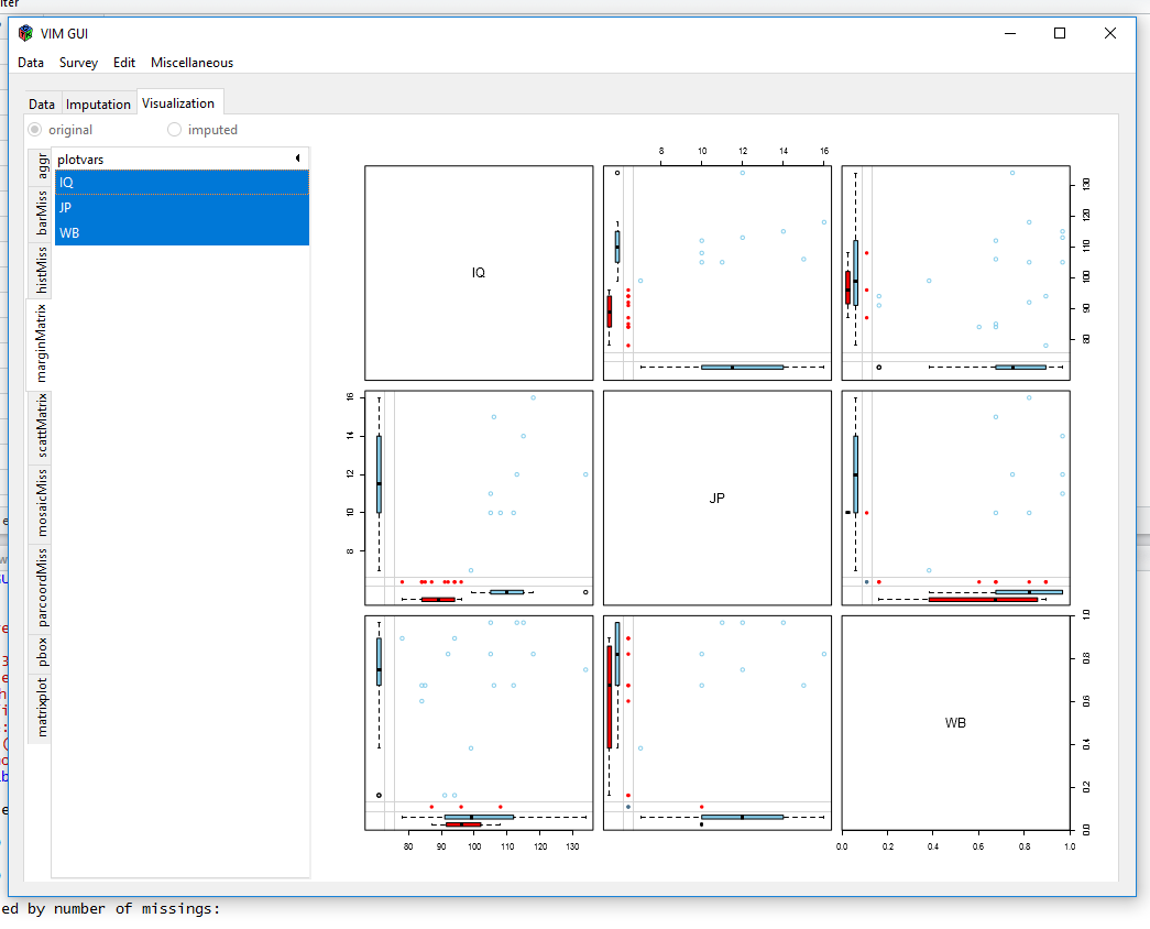
Visualisations like these show you, if there are a lot of different missing data patterns.
The MICE-package can show missingness patterns as well:
install.packages("mice")
library(mice)
md.pattern(EndersTable1_1)
How to use MICE for multiple imputation With MICE you can build an imputation model that is tailored for your dataset. Just use “mice()” with your dataframe and use the defaults of the package.
imp <- mice(EndersTable1_1)
imp
summary(imp)
MICE generates 5 imputated datasets using an algorithm called “predictive mean matching” (pmm), because all data are “numeric” in this case. If there was binary data like a factor with 2 levels MICE would have chosen “logistic regression imputation” (logreg). If there was an unordered factor with more than 2 levels, MICE would have used “polytomous regression imputation for unordered categorical data” (polyreg). And if there were missings in a variable with more than 2 ordered levels, MICE would have used “proportional odds model” (polr).
You can decide for each of your variables which imputation-algorithm is used. There is an easy way to build a “predictor matrix” using quickpred():
predictormatrix<-quickpred(EndersTable1_1,
                           include=c("IQ"),
                           exclude=NULL,
                           mincor = 0.1)
A more tailored imputation model:
set.seed(121012)
predictormatrix<-quickpred(EndersTable1_1,
                           include=c("IQ"),
                           exclude=NULL,
                           mincor = 0.1)
EndersTable1_1<-as.data.frame(lapply(EndersTable1_1,as.numeric))
EndersTable1_1$WB<-as.factor(EndersTable1_1$WB)

imp_gen <- mice(data=EndersTable1_1,
                 predictorMatrix = predictormatrix,
                 method = c('pmm','pmm','polr'),
                 m=10,
                 maxit=5,
                 diagnostics=TRUE,
                 MaxNWts=3000)
How to use Multiple Imputation with lavaan There are three ways to use multiple imputation in lavaan. The first (i) uses runMI() to do the multiple imputation and the model estimation in one step. The second (ii) does the multiple imputation with mice() first and then gives the multiply imputed data to runMI(). Both run the analysis multiple times for each imputed dataset and then use rubins rules to pool the results. Here is a diagram, showing the principle:

The third way (iii) uses the lavaan.survey()-package.
#--------------------------
# Setting up packages
#--------------------------
install.packages("semTools","lavaan")
install.packages("survey")
install.packages("lavaan.survey")
install.packages("mitools")
install.packages("mice")
library("survey")
library("mice")
library("mitools")
library("semTools")
library("lavaan")
library("lavaan.survey")

#--------------------------
# Setting up example data and model
#--------------------------
set.seed(20170110)
HSMiss <- HolzingerSwineford1939[,paste("x", 1:9, sep="")]
randomMiss <- rbinom(prod(dim(HSMiss)), 1, 0.1)
randomMiss <- matrix(as.logical(randomMiss), nrow=nrow(HSMiss))
HSMiss[randomMiss] <- NA

HS.model <- ' visual  =~ x1 + x2 + x3
textual =~ x4 + x5 + x6
speed   =~ x7 + x8 + x9 '
# Variant 1: Imputation and model estimation with runMI
out1 <- runMI(HS.model, data=HSMiss, m = 5, miPackage="mice", fun="cfa", meanstructure = TRUE)
summary(out1)
fitMeasures(out1, "chisq")
# Variant 2: Imputation first, model estimation second with runMI
HSMiss_imp<-mice(HSMiss, m = 5)
mice.imp <- NULL
for(i in 1:5) mice.imp[[i]] <- complete(HSMiss_imp, action=i, inc=FALSE)
out2 <- runMI(HS.model, data=mice.imp, fun="cfa", meanstructure = TRUE)
# Variant 3: lavaan.survey (without weights)
mice.imp2<-lapply(seq(HSMiss_imp$m),function(im) complete(HSMiss_imp,im))
mice.imp2<-mitools::imputationList(mice.imp2)
svy.df_imp<-survey::svydesign(id=~1,weights=~1,data=mice.imp2)
lavaan_fit_HS.model<-cfa(HS.model, meanstructure = TRUE)
out3<-lavaan.survey(lavaan_fit_HS.model, svy.df_imp)
# Variant 4: FIML instead of multiple imputation
out4<-cfa(HS.model, data=HSMiss, missing="FIML", meanstructure = TRUE)FIML is definitely easier to apply than multiple imputation, because you don´t have to work out an imputation model. On the other hand, you can´t specify an imputation model, which could come handy if your data is MAR and you want to include certain auxiliary variables.